Neural Network Decision Boundary

Monday. January 07, 2019 - 6 mins

Inspired by Jon Char's Publication.

Objective

In this post I will implement an example neural network using Keras and show you how the Neural Network learns over time. Keras is a framework for building ANNs that sits on top of either a Theano or TensorFlow backend. I really like Keras cause it’s fairly simply to use and one can get a network up and running in no time. The Keras Blog has some great examples of how to use the framework.

Start off by importing all the required packages

import numpy as np
np.random.seed(0)
from sklearn import datasets
import matplotlib.pyplot as plt
%matplotlib inline

from keras.models import Sequential
from keras.layers import Dense
from keras.optimizers import SGD

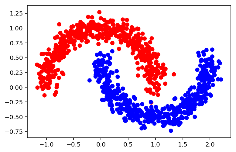
Next we generate the dataset and the scatter plot.

X, y = datasets.make_moons(n_samples=1000, noise=0.1, random_state=0)
colors = ['blue' if label == 1 else 'red' for label in y]
plt.scatter(X[:,0], X[:,1], color=colors)
y.shape, X.shape

((1000,), (1000, 2))

png

Defining the Model

The Keras Python library makes creating deep learning models fast and easy.

The sequential API allows you to create models layer-by-layer for most problems. Keras has different activation functions built in such as ‘sigmoid’, ‘tanh’, ‘softmax’, and many others. Also built in are different weight initialization options. We use the sigmoid activation which limits the values to $[-\epsilon,\epsilon]$

This initialization method corresponds to the 'glorot_uniform' initialization option in Keras.

# Define our model object
model = Sequential()

# kwarg dict for convenience
layer_kw = dict(activation='sigmoid', init='glorot_uniform')

# Add layers to our model
model.add(Dense(output_dim=5, input_shape=(2, ), **layer_kw))
model.add(Dense(output_dim=5, **layer_kw))
model.add(Dense(output_dim=1, **layer_kw))

Defining the Optimizer

While initializing the Keras model we also need to specify an optimizer such as SGD or Adam or RMSProp. In this case we will use SGD. You can however read more about them here.

sgd = SGD(lr=0.001)

Compile the Model

A loss function (or objective function, or optimization score function) is one of the two parameters required to compile a model, the other being the optimizer itself.

model.compile(optimizer=sgd, loss='binary_crossentropy')

Summarize the Model

Keras allows for models to be summarized using model.summary().

model.summary()

_________________________________________________________________
Layer (type)                 Output Shape              Param #   
=================================================================
dense_4 (Dense)              (None, 5)                 15        
_________________________________________________________________
dense_5 (Dense)              (None, 5)                 30        
_________________________________________________________________
dense_6 (Dense)              (None, 1)                 6         
=================================================================
Total params: 51
Trainable params: 51
Non-trainable params: 0
_________________________________________________________________

Train the Model

We can now train our model using the model.fit() method. We will save this as history to refer to it at a future point. Since the number of epochs is very high we will set verbose=0 and shuffle the data as well.

history = model.fit(X[:500], y[:500], verbose=0, nb_epoch=4000, shuffle=True)

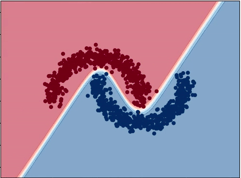
Visualizing the Results

def plot_decision_boundary(X, y, model, steps=1000, cmap='Paired'):
    cmap = plt.get_cmap(cmap)

    # Define region of interest by data limits
    xmin, xmax = X[:,0].min() - 1, X[:,0].max() + 1
    ymin, ymax = X[:,1].min() - 1, X[:,1].max() + 1
    steps = 1000
    x_span = np.linspace(xmin, xmax, steps)
    y_span = np.linspace(ymin, ymax, steps)
    xx, yy = np.meshgrid(x_span, y_span)

    # Make predictions across region of interest
    labels = model.predict(np.c_[xx.ravel(), yy.ravel()])

    # Plot decision boundary in region of interest
    z = labels.reshape(xx.shape)

    fig, ax = plt.subplots()
    ax.contourf(xx, yy, z, cmap=cmap, alpha=0.5)

    # Get predicted labels on training data and plot
    train_labels = model.predict(X)
    ax.scatter(X[:,0], X[:,1], c=y, cmap=cmap, lw=0)

    return fig, ax

plot_decision_boundary(X, y, model, cmap='RdBu')

png

Follow @RohitMidha23

Show some by ing it.

Star